If you have never done it before, inserting a node into a binary search tree might feel a bit intimidating. After all, you need to make sure that it is still a binary search tree once the node is inserted, right? Well, it turns out that you do not need to do anything special to achieve that. The whole process is easier than you think!

Why Would Insertion Be Easy?

Because new nodes are inserted as leaf nodes! This means you do not need to move around any internal nodes. Isn't it great?

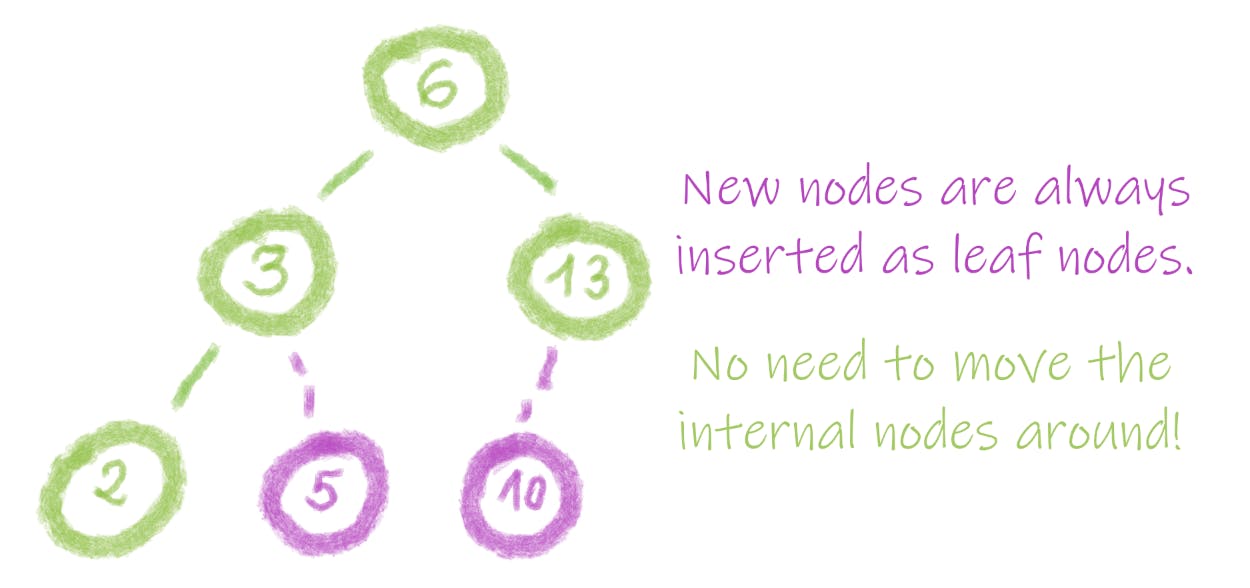
The whole process boils down to:

• finding an existing node to which we can attach our new node - this existing node can be a leaf or any internal node with one child
• inserting the new node

The only thing I can imagine to go wrong here is... messing up inequality signs and thus going right instead of left and vice-versa when walking down the tree. But you must admit that it is a highly unlikely mistake to be done!

So How Do We Code It?

Well, first we need a binary tree node definition. This one should do:

class Node:
  def __init__(self, val, left=None, right=None, parent=None):
    self.value = val
    self.left = left
    self.right = right
    self.parent = parent

If you want, you can drop the reference to parent node - it is not really used for anything useful at the moment. However, it makes life a bit easier when we need to perform other operations like delete. Thus, it is up to you if you want to keep it or not right now.

With the node definition being ready, let's focus on the insertion itself. I am assuming that values in the left sub-tree are always smaller than the one stored in the parent node, thus I am using <. But it is perfectly fine to assume that the right sub-tree values are smaller - just replace both < with <=.

def insert(root, node):
  # 1) Find an existing node to which we can attach our node 
  parent = None
  curr = root

  # We start at the root and continue walking down the tree until we
  # find an appropriate parent for node. We go left or right depends on
  # the new node's value.
  while not curr is None:
    parent = curr
    if node.val < curr.val:
      curr = curr.left
    else:
      curr = curr.right

  # 2) Insert the new node
  # Now that we found an appropriate parent, we update the new node
  node.parent = parent

  # To finish the insertion, we also need to update the parent node itself.
  # If parent is None, the tree is empty and our node becomes the root.
  # Otherwise, depends on the node's value, we set it to be parent's left
  #  or right child
  if parent is None:
    root = node
  elif node.val < parent.val:
    parent.left = node
  else:
    parent.right = node

  return root

What About The Time Complexity?

The function mostly consists of assignments and if-else statements which are O(1). Unfortunately, our complexity is higher than that because we also have a while loop that we use to walk down the tree.

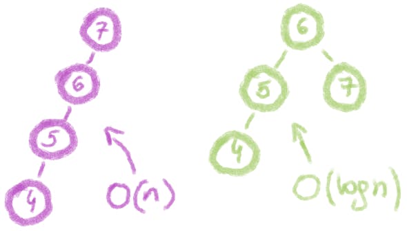
And how many times is the while loop executed? It depends on the shape of our tree.

If we are unlucky and the tree is a one long branch, we may need to go through all n nodes to find the right spot. Thus, the time complexity is O(n).

For a perfectly balanced tree, the tree height is log(n). This means that even if we need to get to the very bottom, we visit only log(n) nodes which gives us O(logn).

So which complexity should we go for? In general, randomly built binary search trees are expected to have height of log(n), so O(logn) is the answer. But if you are not convinced, check out the beautiful math-based proof included in Introduction To Algorithms by Thomas H. Cormen, Charles E. Leiserson, Ronald L Rivest, Clifford Stein (Chapter 12.4 Randomly built binary search trees). It is hard to argue with those guys!

---

The cover image was created with the help of Freepik